Excel has several functions that can return information from your own custom tables in many different ways. Here are some of the most common functions, followed by some examples on how to use them:

VLOOKUP(value,range,columnindex,sorted)

This function searches for a given value down the rows in the first column in the given range, and returns the content of the cell in the indicated column.
value : the value you want to find in the table, may be a string, number or a cell reference.
range : the address to the range containing the custom table, or a user-defined name.
columnindex : the column number in the table that you want to return the value from.
sorted : optional logical value, TRUE or FALSE. If left out the argument defaults to TRUE and the function assumes that the values in the first column in the table range is sorted in ascending order. If the argument is set to FALSE the content in the first column can be sorted in any order, and the function will return an error if the lookup value is not found.

Note! The argument sorted works only in Excel 5.0 or later. Older versions assumes that the values in the first column is sorted in ascending order.

HLOOKUP(value,range,rowindex,sorted)

This function searches for a given value from left to right in the first row in the given range, and returns the content of the cell in the indicated row.
value : the value you want to find in the table, may be a string, number or a cell reference.
range : the address to the range containing the custom table, or a user-defined name.
rowindex : the row number in the table that you want to return the value from.
sorted : optional logical value, TRUE or FALSE. If left out the argument defaults to TRUE and the function assumes that the values in the first row in the table range is sorted in ascending order. If the argument is set to FALSE the content in the first row can be sorted in any order, and the function will return an error if the lookup value is not found.

Note! The argument sorted works only in Excel 5.0 or later. Older versions assumes that the values in the first row is sorted in ascending order.

INDEX(range, rowindex,columnindex)

This function returns the value from the cell in the range according to the given row- and column indexes.

Examples:

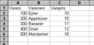
Assume that you have the following table in a worksheet:

Function	Returns
=VLOOKUP(200,A2:C6,2)	Appelsiner
=VLOOKUP(400,A2:C6,3)	12
=VLOOKUP(350,A2:C6,2)	Bananer

If the lookup value is not found, the function returns the value from the largest value that is less than the lookup value. This can be useful when you want to look up values within preset intervals, e.g. a list of discount rates for different purchase amounts.

=VLOOKUP(350,A2:C6,2,FALSE) will return the error #N/A.
If you set the argument sorted to FALSE and the lookup value is not found, the function will return the error #N/A (not available).

=HLOOKUP("varenavn",A1:C6,3,FALSE) will return Appelsiner (oranges).

=HLOOKUP("varenavn",A1:C6,10,FALSE) will return the error #REF!
In this case the row reference is too large, the matrix contains only 6 rows, and it's not possible to return values from outside the given matrix.

=INDEX(A2:C6,2,3) will return 15.

The functions VLOOKUP() and HLOOKUP() can be used together with the ROW() or COLUMN() functions to avoid several manual corrections of row- or columnreferences when copying the lookup-functions.

Examples:

Select cell D5 and enter the following formula:
=VLOOKUP($A$1,$F$10:$O$100,COLUMN()-2,FALSE)
This formula can now be copied from cell D5 and all the way to cell L5. Now you will get in return the values from the table in the r F10:O100 (except the lookup values in the first column) matching the lookup value given in cell A1.

Like this post